© 2022.

This work is licensed under a Creative Commons Attribution 4.0 International License.
© 2022.
This work is licensed under a Creative Commons Attribution 4.0 International License.
This page serves as companion website for the MMSP 2022 paper:
F. Simonetta, S. Ntalampiras, and F. Avanzini “Acoustics-specific Piano Velocity Estimation,” MMSP, 2022 link.
Motivated by the state-of-art psychological research, we note that a piano performance transcribed with existing Automatic Music Transcription (AMT) methods cannot be successfully resynthesized without affecting the artistic content of the performance. This is due to 1) the different mappings between MIDI parameters used by different instruments, and 2) the fact that musicians adapt their way of playing to the surrounding acoustic environment. To face this issue, we propose a methodology to build acoustics-specific AMT systems that are able to model the adaptations that musicians apply to convey their interpretation. Specifically, we train models tailored for virtual instruments in a modular architecture that takes as input an audio recording and the relative aligned music score, and outputs the acoustics-specific velocities of each note. We test different model shapes and show that the proposed methodology generally outperforms the usual AMT pipeline which does not consider specificities of the instrument and of the acoustic environment. Interestingly, such a methodology is extensible in a straightforward way since only slight efforts are required to train models for the inference of other piano parameters, such as pedaling.
The code is available at https://github.com/LIMUNIMI/ContextAwareAMT
The source dataset was Maestro and was used as provided by ASMD library. The Maestro dataset was selected using the ASMD Python API; then, train, validation, and test splits were partitioned in 6 different subsets, each associated to one of the presets in Table I (see paper), for a total of 6 × 3 = 18 subsets. From 18 subsets, 6 sets were generated by unifying subsets associated to the same preset, so that each set was still split in train, validation, and test sets. Each generated set was resynthesized and saved to a new ASMD definition file.
The 6 new subsets in each split were chosen as follows. First, one split at a time among the already defined train, validation, and test was selected. Supposing that the chosen split has cardinality K, C clusters were created with C = ⌊K/6 + 1⌋ and a target cardinality t = 6 was set. Then, a redistribution policy is applied to the points of the clusters: for each cluster with cardinality < t – a “poor” cluster – we look for the point nearest to that cluster’s centroid and belonging to a cluster with cardinality > t – a rich cluster – and move that point to the poorer cluster. The redistribution stops when all clusters have cardinality ≥ t. Since the redistribution algorithm moves points from rich clusters to the poor ones, we named it “Robin Hood” redistribution policy. Having obtained C clusters each with 6 samples, we partitioned the chosen split in 6 subsets as follows:
we randomized the order of subsets and clusters
we selected one point from each cluster using a random uniform distribution and assigned it to the one of the 6 subsets
we did the same for the other 5 subsets
we restarted from point 2. until every point is assigned to a cluster.
Clustering was performed as follows: first, a set of features was extracted from the recorded MIDI of each music piece available in Maestro in order to describe the available ground-truth performance parameters. Namely, the velocity and pedaling values were extracted for a total of 4 raw features – i.e. 1 velocity + 3 pedaling controls. For each raw feature, 3 high-level features were computed by fitting a generalized normal distribution (N) and obtaining its parameters (α, β, and μ). Another high-level feature was computed as the entropy of each raw features (H). Finally, for each pedaling MIDI control, the ratio of 0-values and 127-values was added (Q); this feature is meaningful because most of the research about piano pedaling transcription considers the pedaling as an on-off switch, even if in real pianos it can be used as a continuous controller. Overall, each Maestro music piece was represented by concatenating the high-level features, including 3 × 4 features N, 4 features H, and 2 × 3 features Q, totaling 22 features. Then, PCA was performed to identify 11 coefficients while retaining 89%, 93%, and 91% of variance for the train, validation and test splits. Isolation Forest algorithm with 200 estimators and bootstrap were also employed to detect potential outliers, resulting in 81, 39, and 36 removed points from the train, validation, and test splits. Finally k-means clustering with kmeans++ initialization routine was applied to find C centroids in the data with the outliers removed; from the found centroids, C clusters were reconstructed from the full dataset (outliers included).
NMF has largely been used for score-informed AMT and our application is mainly based on the existing literature. Using NMF, a target non-negative matrix S can be approximated with the multiplication between a non-negative template matrix W and a non-negative activation matrix H. When applied to audio, S is usually a time-frequency representation of the audio recording, W is the template matrix representing each audio source, and H represents the instants in which each source is active. As such, the rows of W represent frequency bins, the columns of W and the rows of H refer to sound sources, and the columns of H are time frames. The W and H matrices are first initialized with some initial values and then updated until some loss function comparing S and W × H is minimized.
The proposed method for NMF is shown in figure 1 (see paper). Similarly to previous works we split the temporal evolution of each piano key in multiple sectors, namely the attack, the release, and the sustain. Each sector can be represented by one or more columns in W (and correspondingly rows in H). We used the following subdivision:
 |
|---|
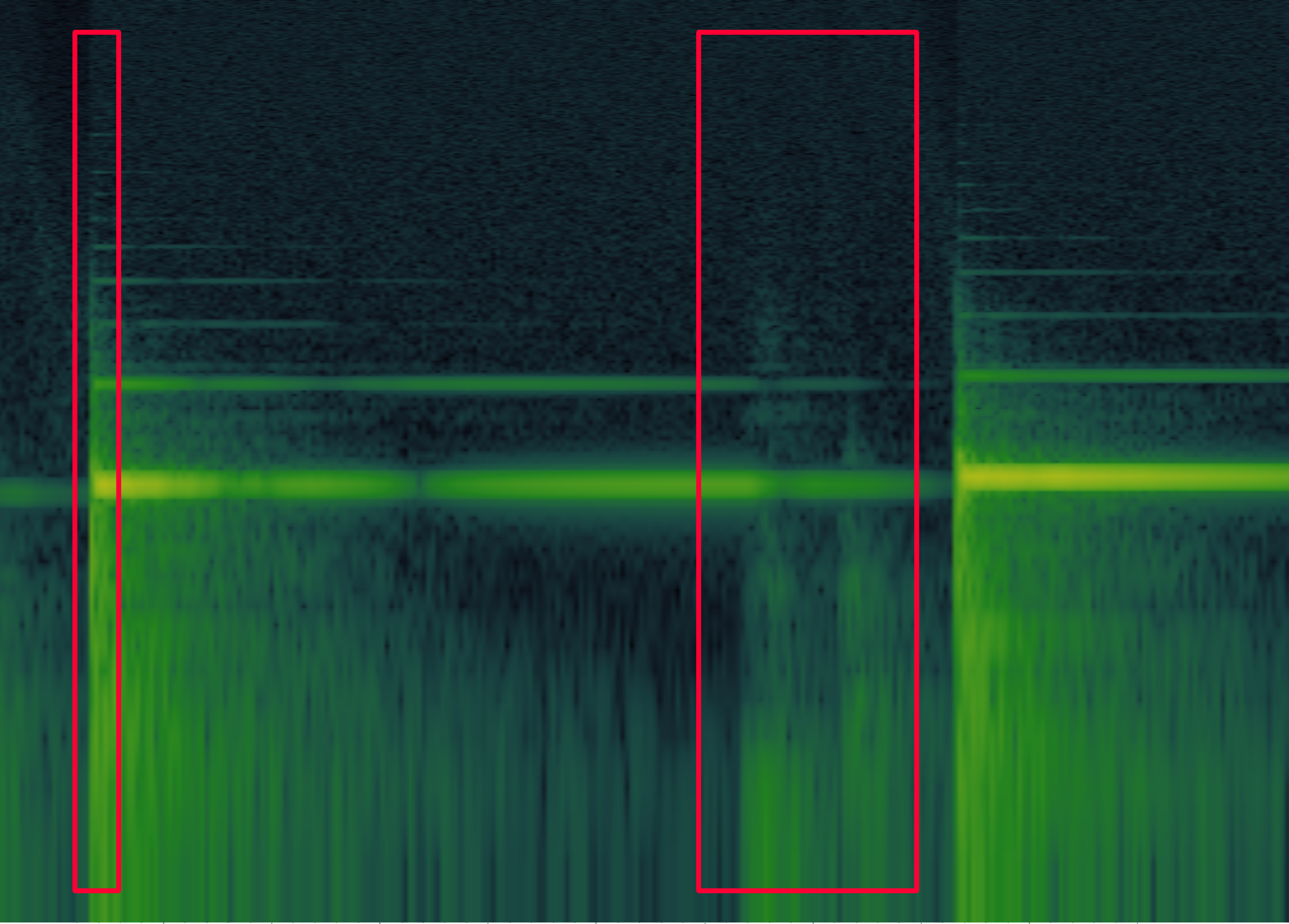
| Figure I: Log-Spectrogram of a piano note. The two red rectangles highlight the impulse connected with the attack of the note, and the impulses connected with the hammer release of the note. The image was obtained using Sonic Visualizer and the audio scales synthesized with Pianoteq “Steinway B Prelude” used for the computation of the initial NMF template. The Sonic Visualizer project used for extracting this image is available in the online repository. The spectrogram has been computed using windows of 1024 frames and 50% of overlap; the intensity scale is in dB, while the frequency scale is logarithmic; no normalization was applied. The pitch is 73, velocity is 22, and duration is 1.5 seconds. |
1 column for the attack part, representing the first frame of the note envelope (∼ 23 ms)
14 columns for the sustain section, representing 2 frames each; if the note sustain part lasts more than the 28 frames (∼ 644 ms), the remaining part is modeled with the last column;
15 columns for the release part(∼ 345 ms), starting from the recorded MIDI offset and representing one audio frame each; the reason is that, as shown in Figure I, after the MIDI offset, there are still about 350 ms before the hammer comes back, producing a characteristic impulsive sound and definitely stopping the sound.
The initial W matrix is constructed by averaging the values obtained from a piano scale synthesized with pycarla and Pianoteq’s “Steinway B Prelude” default preset. The scale contained all 88 pitches played with 20 velocity layers, 2 different note duration – 0.1 and 1.5 seconds – and 2 different inter-note silence duration – 0.5 and 1.5 seconds. First, the amplitude spectrogram is computed using the library Essentia . We used 22050Hz sample-rate, frame size of 2048 samples (93 ms), hop-size of 512 samples (23 ms), and Hann window types.
The initial H matrix, instead, is generated from the perfectly aligned MIDI data, by splitting each pitch among the various subdivisions as explained above.
Finally, the NMF optimization is performed using Euclidean distance and multiplicative updates . Our NMF optimization routine is adjusted as follows: a first step (A) is performed separately on 5 windows with no overlap and with H fixed; splitting the input activation matrix and the target spectrogram in windows is beneficial because the multiplicative contribute for W depends on S**HT , which can be repeatedly adjusted on each window, increasing both accuracy and generalization of the W estimation. Having slightly optimized W, we applied the second step (B), consisting in 5 iteration of the usual NMF. Before both step A and B, W and H were normalized to the respective maximum value so that their values lay in [0,1].
Once the NMF algorithm is finished, we use the original perfectly aligned activation matrix to select the region of a note in H and W to obtain its approximated spectrogram separated from the rest of the recording. We consider the first 30 frames (690 ms) of each note, padding with 0 if the note is shorter. We finally compute the first 13 MFCC features in each column of the spectrogram using Essentia.